The Identification of Travelling Waves in a Voltage Sensor Signal in a Medium Voltage Grid Using the Short-Time Matrix Pencil Method

The Omicron-Lab Bode 100 vector circuit analyzer provided by DACPOL SP was used in the research. Z O.O.

Abstract

Most of the fault wave localization methods are based on the analysis of line current transformed by current transformers and are limited to high voltage grids. Fault wave localization in medium voltage grids is still being developed. This paper presents a new real-time algorithm for the identification of travelling waves in a distribution grid using voltage signal and the short-time matrix pencil method. To obtain the secondary side voltage waveforms at substation, the model of a resistive voltage sensor based on the broadband measurements from 10 Hz to 20 MHz was developed. The tested sensor amplifies the frequencies associated with travelling waves more than utility frequency allowing for the identification. Short-circuit simulations on the IEEE 34-bus feeder was performed to test the algorithm. The developed method can detect even the waves of low amplitude.

1. Introduction

Protecting the power system from faults is one of the objectives of protective relaying. Fast removal of disturbance limits the damage inflicted on power equipment and reduces its negative impact on the quality of electric power. Therefore, the development of fast and accurate relays and fault locators in distribution grids is a key issue from both a technical and an economic point of view. In case of high voltage networks, localization of faults is easy as they are characterized by a large dispersion of measurements and loop structure. In case of distribution networks measurements are mainly made at a single point of the substation there. Moreover, distribution grids are of a tree structure, which makes faulted branch identification uncertain. The solution to this problem may be the use of travelling wave locators, which in this case may be more precise than conventional methods. In order to make the use of such locators possible, it is necessary to develop the most accurate methods of travelling wave identification.

The conventional approach to fault detection is based on the analysis of currents and voltages of a fundamental frequency. For this reason, protection algorithms based on these types of signals require the analysis of a signal interval that is long enough to make sure that the disturbance has occurred. A more modern approach is based on travelling waves, which are higher frequency signals propagating along power lines. This type of protection is sometimes called “ultra-high-speed”. It detects current and voltage waves generated by faults. Then, this protection determines both the type and location of the disturbance on the basis of the comparison of their amplitudes and arrival times to the measuring devices. Undoubtedly, the key advantage of the wave-based protection is the speed of operation (less than 4 ms). Moreover, it works correctly with series-compensated transmission lines and during power swings.

The fault location using travelling waves can be divided into two-terminal and single-terminal schemes. In case of double-terminal relays, the measurement data acquisition occurs at the ends of protected lines and it requires transmission of measurement data between devices. However, single-terminal relays analyse the signals of currents and voltages from only one measurement point. It needs to be highlighted that two-terminal relays are characterized by higher reliability because they use waves directly generated by the disturbance to localize and classify it. These waves have the highest possible amplitude and are detected first after a fault. However, in case of single-terminal relays, the protection is based on the wave generated by the disturbance and on the waves reflected from line discontinuities, branches and the fault itself. It is due to the lack of a second measurement point in the network.

High voltage grids are characterized by the presence of substations with metering equipment at the line ends. Double-terminal relays are therefore used here. In the case of distribution networks, high/medium voltage substations are usually the only place where protection relays with transformers or sensors are placed. This means that in distribution networks using single-ended wave relays is the cheapest solution.

Distribution grids are the networks with a tree topology, and this feature makes accurate fault location difficult. For both conventional and wave locators of faults the situation is more complicated than in transmission networks, as several potential faulted branches may exist at a known distance from the substation. Only one of the branches is faulted. However, a short-circuited line can be determined by comparing the amplitudes of the current waves scattered on the substation buses.

Different methods of locating faults have been proposed, such as detection of frequencies associated with wave oscillations between nodes, comparison of the measured current with predicted one for a given short-circuit location and more traditional methods based on detection of fault wave fronts. The following methods have been used to detect wave fronts: wavelet transform, principal component analysis based on feature extraction, Teager energy operator, ensemble empirical mode decomposition and the matrix pencil method, which is discussed and used in this paper. The matrix pencil method is used to decompose a signal into the sum of exponentially damped sinusoids. In the field of electrical power engineering, the matrix pencil method has been used to estimate the fundamental modes of oscillations due to faults and to estimate harmonics and subharmonics.

Electrical signals processed by digital data processing algorithms are delivered to the relay by the means of measuring devices located on the station. These devices include current and voltage transformers, Rogowski coils or sensors reducing the level of electrical signals to the level acceptable by the relays. It is important that the signal on the secondary side of these devices is reproduced as accurately as possible and ideally it should only be scaled. In practice, however, the measuring instruments have variable gain and phase shift depending on the signal frequency. High frequencies should not be attenuated by the instrument too much in order to be able to detect an incoming travelling wave, which is a fast-changing waveform and therefore contains high-frequency components. It needs to be stressed that in order to reproduce the amplitude of the fault wave accurately, instrument should introduce a constant time delay (preferably none at all) and its amplification characteristics should be as little variable as possible.

Transformers are the instruments that are traditionally used in the electric power industry to measure voltage. They are characterized by a very precise transformation of electrical signals, but they also have disadvantages. They contribute to the negative phenomenon of ferroresonance, are exposed to damages caused by short circuits in the secondary circuit and are not able to transform high-frequency (>3 kHz) voltage components precisely. That is why, unconventional sensors based on the mechanisms different from the transformer system have been developed as the response to the need to measure transient components accurately.

For voltage measurements, voltage sensors based on capacitive (C), resistive (R) and resistive-capacitive (RC) dividers are popular unconventional sensors. In particular, R and RC dividers are the most popular ones as they are unable to induce ferroresonance due to negligible inductance, transform transients and high frequencies accurately, allowing for the discharge of accumulated charge on the line and are resistant to secondary side short circuits. These dividers can be successfully used for power quality measurements and for short-circuit location using wave phenomena.

The literature on the modelling of conventional transformers is vast but, unfortunately, usually refers to the description of their characteristics at the frequencies below 10 kHz. Moreover, the authors have not been able to find the numerical data of the Bode plots or transfer functions of voltage transformers (both conventional and unconventional) up to 1 MHz even in the articles describing the studies in this field. Such data are available for a conventional current transformer. Of course, sensors differ in design, leading to variations of their transfer characteristics from one type to the another but knowing the transfer function of an example one seems needed.

In order to obtain such data, measurements of the frequency characteristics of a medium voltage sensor were made. Then, they were used to develop its transfer function model. The improved short-time matrix pencil method was then presented in application to the detection of voltage short-circuit waves in the medium voltage network measured on the secondary side of voltage sensors.

The structure of the paper is as follows. Section 2 provides a description of short-time matrix pencil method with its application for finding signal pulses. There is also provided the algorithm for identification of the pulses. Section 3 contains measurement results of voltage sensor transfer function and results of the algorithm's operation on the basis of conducted simulations. Conclusions are given in Section 4.

2. The Identification of Fault Impulses in a Medium Voltage Grid

2.1. The Short-Time Matrix Pencil Method

The short-time matrix pencil method (STMPM) approximates a signal inside the window that moves with time as the sum of sinusoidal components with an exponentially variable amplitude:

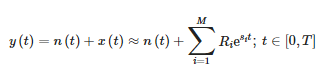
where:

• y(t)—measurement signal,
• n(t)—noise,
• x(t)—original signal,
• Ri—residua or complex amplitudes of components,
• Si—complex poles and
• M—number of approximation components.

For a sampled signal t = kT_s, the above equation takes the following form:

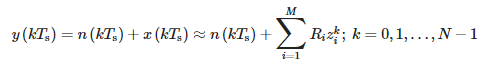
where:

• Ts—sampling period and
• N—number of samples.

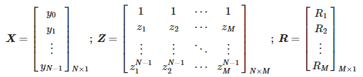
In order to determine the approximation parameters, the following matrix shall be constructed:

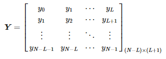
Here, L is a pencil parameter. The number of approximation components M satisfies the following relation:

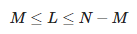
Thus, we see that the maximum value of M is equal to ⌊N/2⌋.
By subjecting the matrix Y to singular value decomposition (SVD) we obtain:

where:

• U—unitary matrix of (N - L) x (N - L) size,
• Σ—rectangular diagonal matrix of singular values with size of (N - L) x (L + 1) and
• V—unitary matrix of (L + 1) x (L + 1) size.

If the measured signal contained no noise, the Σ matrix would contain exactly M non-zero singular values. Due to the noise, the singular values can be distorted, which manifests itself by additional small singular values. The noise effect is eliminated by removing these small values. Only M dominant values are left that satisfy the following condition:

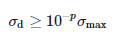
where σ_max is a dominant singular value and p is the number of accurate significant decimal digits of measurement.

Then sub-matrices of the resulting SVD matrices are constructed:

1. Matrix U'=[u1,u2,…,u_M] of size (N - L) x M is created by leaving columns corresponding to the singular values satisfying Condition (7) and removing the others;
2. Square diagonal matrix Σ=diag(σ1,σ2,…,σM) is formed by removing the columns and rows of the Σ matrix, which contain singular values that do not satisfy Condition (7);
3. Matrix V'=[v1,v2,…,v_M] of size (L + 1) x M is formed by leaving the columns corresponding to the singular values satisfying Condition (7) and removing the others.

Then, the matrix V₁' is created by removing the last row of V' matrix. V₂' is built by removing the first row of V' matrix.

Then, the following matrices are calculated:

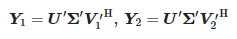
Values zi are non-zero generalized eigenvalues of matrices pair (Y₁, Y₂), namely eigenvalues of Y^†₁Y₂, where Y^†₁ is Moore–Penrose pseudoinverse of Y₁. Then we calculate poles:

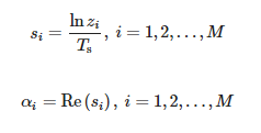
The values of the amplitudes can be determined as follows:

where:

The above operations are performed in the short-time matrix pencil method for successive intervals of data.

The approximate results of eigenvalues, pseudoinversions and SVD algorithms can affect emerging of zi non-zero though close to zero values. These values affect the MPM speed and can adversely affect their results, so it is worth removing them before calculating the residues.

2.2. The Behaviour of the Component Poles in the Vicinity of a Pulse

Faults in the electrical grid generate pulses propagating along power lines at the speeds close to the speed of light. These impulses can be identified using pole shift analysis of the STMPM approximation. Figure 1 shows three example Gaussian-shaped pulses and the poles of their approximation with STMPM. When the pulse comes, the approximation with exponential components changes as the time window moves. When the pulse is to the right of the middle point of the window the poles of the approximation have a positive real part, when the Gaussian vertex is in the middle of the window the real part of the poles is close to zero, and when the pulse is in the first half of the window the poles have a negative real part. The change in the sign of the real part of the poles therefore indicates that the centre of the pulse has passed through the middle point of the sampling window. We can also see from Figure 2 that the poles with the largest absolute value of the real part (and therefore with the fastest amplitude changing rate) have the largest value of the initial amplitude modulus (residuum).

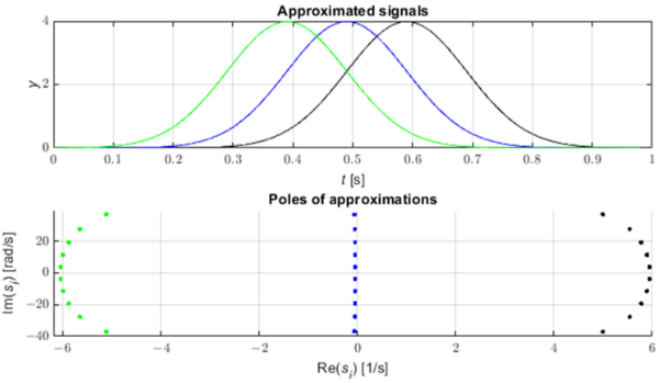
Figure 1. Gaussians and corresponding poles of approximations.

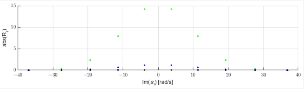
Figure 2. Residues of components of Gaussian approximations.

Thus, we see that the time coordinate of the pulse top can be approximately identified with the moment of change of the sign of the damping coefficients.

Obtaining the time-dependent course of these coefficients with the use of STMPM, we can subject them to linear approximation in the vicinity of the point where the coefficients pass through zero and obtain an approximate pulse top coordinate. It should be noted that the coefficients characterized by the highest variability are also characterized by the highest amplitude—they are the largest components of the pulse.

2.3. The Real-Time Pulse Detection Algorithm

The flowchart of the algorithm for the detection of impulses originating from travelling waves is presented in Figure 3. The algorithm subjects successive windows of the signal to STMPM in order to extract decay rates of the approximation components.

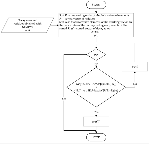
Figure 3. The algorithm of selection of decay rates.

The obtained components are subjected to selection, the procedure of which is presented in Figure 4. The selection is based on the assumption that those components of the STMPM, which are characterized by the largest amplitude, should be taken for the peak time approximation—they constitute the largest contribution to the transient component of the signal. This is in agreement with the observation from the previous point—the components with the largest amplitude variation are characterised by the largest initial amplitude. In the case when the component with the largest amplitude is characterized by small decay rate during the whole window of length T_w—smaller than the parameter c—or its maximum contribution to the signal is smaller than r, the next component in terms of amplitude magnitude is selected as a potential candidate for the decay rate α. By repeating this procedure for subsequent components until the condition is met, one finally obtains the coefficient α that is used then to approximate the pulse arrival time. If none of the components satisfy the above conditions, the one with the highest amplitude is selected.

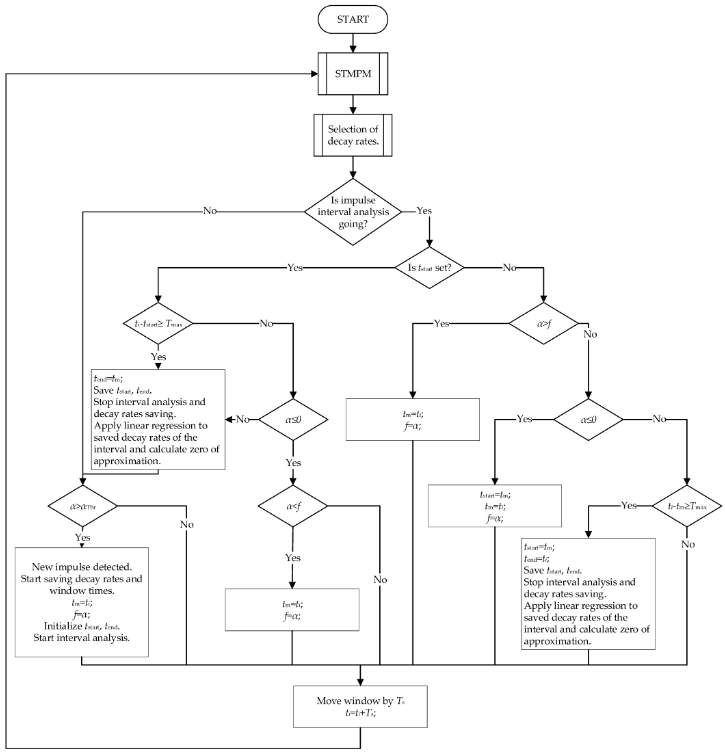
Figure 4. The algorithm of pulse identification.

The time associated with a window is considered to be:

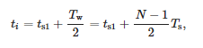
where t_s1—time of first window sample and T_w—window width.

The arrival of a pulse is indicated by a sharp increase in the α rates associated with a rapid change of the signal at the end of the sampling window. The parameter α_Thr is selected as the threshold of decay rates. When the detection threshold is exceeded, the subsequent values of α coefficients and window times are written to memory, and data analysis is started to determine more accurate pulse boundaries. The moment t_start with the highest value of α before changing the sign of the decay rate is selected as the proper start of the pulse. In order to store the potential times of the correct pulse boundaries, the variable t_m was introduced with the variable f containing the largest values of α of the pulse calculated so far.

If the value of t_start is found, the search for the final proper end of the pulse t_end starts. This corresponds to the smallest value of α before the sign changes again, this time to the positive one. The variable i_m is used again to store the previous potential endpoints. The variable f contains the previous minimum α values.

When the pulse length is equal to the T_max of the samples or the end of the pulse is found, the analysis of the pulse is terminated.

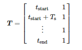
Function α(t) in the interval [t_start; t_end] is subjected to linear regression. The coefficients of this regression are found as the solution to the following problem:

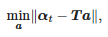
where: α_t=[α(t_start),α(t_start+Ts),…,α(t_end)]^T, a=[a₁,a₀]^T

The sought coefficients are:

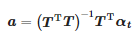
Whereas the moment of arrival of the impulse is:

2.4. The Adapted IEEE 34-Bus Test Feeder

For short-circuit calculations, a 34-bus IEEE test feeder model in Simulink was created. The topology of the feeder is shown in Figure 5. The feeder is based on a real network in the state of Arizona. It is simple enough not to become a substantial computational burden during transient simulations with small integration step. The model was simplified, and the parameters changed to imitate the European grids:

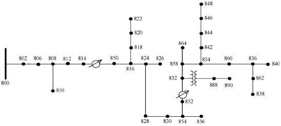
Figure 5. The IEEE 34-bus feeder topology.

• Grid voltage was changed from 24.9 kV to 16.5 kV;
• All sections of power lines were assumed to be overhead lines with the same parameters;
• Voltage regulators were removed;
• The distributed loads were assumed to be lumped at buses at the far end of the loaded lines;
• Loads were connected to the medium voltage grid via distribution transformers;
• High/medium voltage transformer neutral point was disconnected from grounding.

Voltage source parameters:

• 50 Hz frequency;
• 115.5 kV line voltage;
• Resistance 0.00227 Ω.
• Symmetrical source with phase shift of L1 phase equal to 0°.

Parameters of power transformer:

• Voltage ratio 115.5/16.5;
• Vector group of high voltage winding Yg;
• Vector group of low voltage winding D11;
• Power 6.3 MVA;
• Relative short-circuit voltage 7.5%;
• Short-circuit resistance equal to 0.49% of equivalent impedance.

Parameters of distribution transformers:

• Voltage ratio 15.75/0.4;
• Vector group of high voltage winding D11;
• Vector group of low voltage winding Yg;
• Power 630 kVA;
• Relative short-circuit voltage 6%;
• Short-circuit resistance equal to 17.2% of equivalent impedance.

Parameters of power lines:

• Three-phase line without neutral;
• One conductor per phase;
• Conductor diameter 0.8466 cm;
• T/D ratio 0.311;
• DC resistance 0.5939 Ω/km;
• Horizontal positions of conductors x=[-1.05, 0, 1.05];
• Vertical positions of conductors u=[-9.05, 10.61, 9.05];
• Ground resistivity ρ=100 Ωm.

Capacitances were attached to each transformer as shown in Figure 6 in order to model the properties of the transformers at high frequencies.

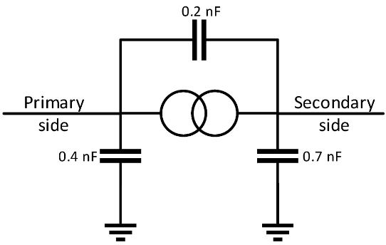
Figure 6. Transformer model.

Power lines were modelled between 1 Hz to 1 MHz taking into account the skin effect using the Universal Line Model.

Simulations of single-phase and multiphase short circuits with zero crossing resistance were performed at 20%, 50%, 80% and 100% length of lines. It corresponds to 76 short-circuit locations. The integration step of the simulation was Δt=0.1 μs. Tustin/Backward Euler was the used method of integration.

3. Results

3.1. Measurements of the Transmission Characteristics of the Medium Voltage Sensor

The measurements of the frequency response were carried out for a medium voltage sensor intended for mounting in connector heads. The sensor was a resistive divider with a rated primary voltage of 20/√3 kV and rated secondary voltage of 3.25/√3, which corresponds to the voltage ratio of:

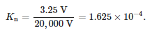
The OMICRON Lab’s Bode 100 vector network analyser was used for the measurements. This device makes the measurements in the range from 1 Hz to 50 MHz possible. The gain and phase measurement function of the device was used to carry out the tests. This function was based on the comparison of the amplitude and phase of the voltage signals on the primary and secondary sides of the sensor. The transfer function measurement, defined as the ratio of the voltage on the secondary side to the voltage on the primary, side was performed for 2048 frequency values in the range from 10 Hz to 20 MHz. The measured values are presented in Figure 7.

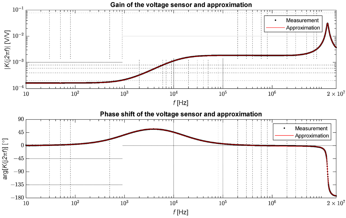
Figure 7. Measurement results of the transmittance of the medium voltage sensor.

The tested voltage sensor maintains a nominal transfer coefficient for signals up to the frequency of about 1 kHz, then the plot rises to the gain level of about 1.84 x10^-3; this level is maintained between from about 12.5 kHz to 6.6 MHz. Due to differentiating property of the sensor, here is a positive phase shift of approximately 57° in the transition zone from 100 Hz to 100 kHz. In the case of phase, we can distinguish two zones for which the offset does not exceed 6°. In this case, the frequency range is up to approximately 130 Hz and from 105 kHz to 9.4 MHz. Therefore, it can be concluded that in the range from 105 kHz to 6.6 MHz, and the signals are proportionally transformed but with a different proportionality factor than near the network frequency. In the case of wave phenomena, this range is sufficient to represent the shape of the waves propagating in a grid accurately. It is worth noting that voltage sensors with different constructions can exhibit different transfer properties.

In order to develop a mathematical model of the sensor, the “tfest” function of MATLAB was used to approximate the data obtained by a stable transfer function of the following form:

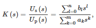
where:

• Up(s) —voltage on the primary side of the sensor,
• Us(s) —voltage on the secondary side of the sensor,
• n —the order of numerator,
• m —the order of denominator and
• ak, bl —coefficients of polynomials of the denominator and numerator of the transmittance, successively.

The values of the transfer function coefficients are presented in Table 1. It is worth noting that the modelled transmittance is proper as the order of the denominator is greater than the order of the numerator. Figure 7 also presents the comparison of the transfer functions obtained from measurements with the approximation by Formula (19). The mean square error between measurement points and the approximation determined by the following relation was also calculated:

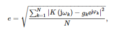
where:

• N = 2048—number of measurement frequencies
• g_k —measured gain of the sensor at pulsation ω_k and
• φ_k —measured phase shift of the sensor at pulsation ω_k.

The approximation error value is equal to:

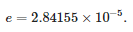
Table 1. Values of polynomial coefficients of the equivalent transmittance of a voltage sensor with resistive divider structure.

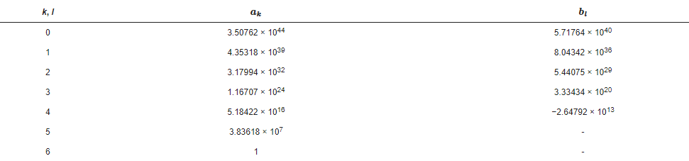
Figure 8 shows the comparison of the phase voltage waveform at the substation obtained from the simulation and the voltage at the output of the modelled sensor in the case of a direct three-phase short circuit with the earth at node 816. It is clearly visible that the amplification of fast transients is greater than slow transients. It is worth noting that these waveforms are amplified almost proportionally.

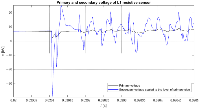
Figure 8. Comparison of the phase voltage waveform (v_L1) and the voltage at the output of the sensor scaled to the primary voltage (v_L1/K_n) during fault.

3.2. The Identification of Short-Circuit Impulses Using STMPM

Figure 9 shows the waveform of all decay rates of an example voltage waveform at a substation after a three-phase zero impedance short circuit to earth at node 816 of the model. It can be seen that the lack of selection of decay rates makes pulses difficult to locate; this is particularly true for weaker pulses. On the other hand, the visual observation of the decay rates allows for the easy identification of intervals containing pulses in the case of visual analysis of phase voltage waveforms, although this is not always easy in the case of small pulse amplitudes.

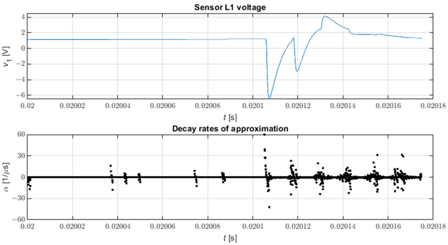
Figure 9. All decay rates of STMPM approximation. N = 9, L = 4.

Figure 10 shows the selected decay rates together with the linear regression used to identify the moment of pulse arrival. The number of false pulse detections can be reduced by filtering out unnecessary attenuation coefficients.

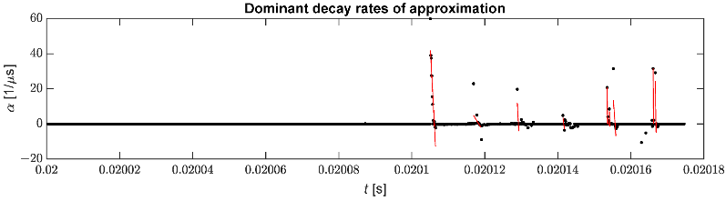
Figure 10. Selected decay rates used for pulse identification.

Table 2 shows the errors in identifying the arrival time of the first incoming wave at the station. This error is defined by the following equation:

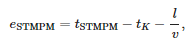
where:

• t_STMPM —arrival moment according to STMPM,
• t_K —fault moment,
• l —distance of the short-circuit location from the substation and
• v = 299,552,300 m/s—propagation speed of fault waves measured for a short circuit at the furthest node (838).

The method parameters used to obtain the results are:

• N = 5—number of samples per time window;
• L = 2—pencil parameter;
• p = 6—the number of accurate significant decimal digits of measurement;
• α_Thr=1051s —pulse detection threshold;
• T_max=2.1 μs —maximum pulse width;
• T_w=0.5 μs —window width;
• T_s=0.1 μs —sampling period;
• r=0.02 V —amplitude threshold.

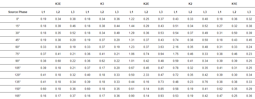
Table 3 shows the standard deviations of the temporal error of the pulse.

Table 2. Temporal error of wave identification in case of different faults. Unit: µs. K3E—three-phase-to-ground fault, K3—three-phase fault, K2E—two-phase-to-ground fault, K2—two-phase fault, K1E—phase-to-ground fault.

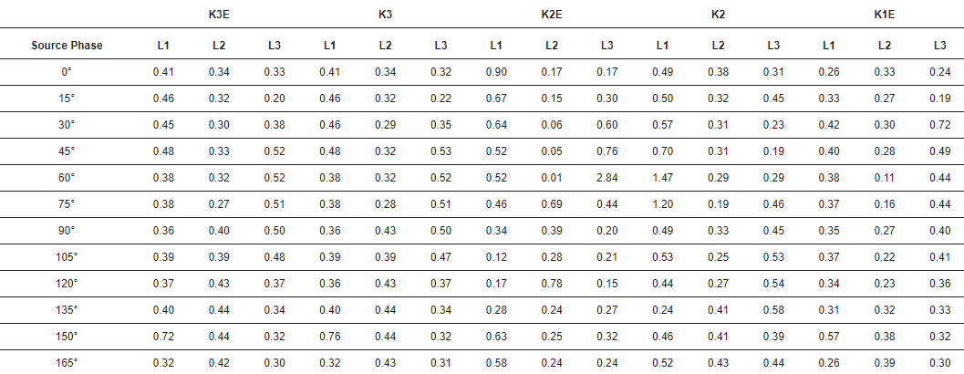
Table 3. Standard deviation of temporal error. Unit: µs. K3E—three-phase-to-ground fault, K3—three-phase fault, K2E—two-phase-to-ground fault, K2—two-phase fault, K1E—phase-to-ground fault.

4. Discussion

The transfer function model of a resistive voltage sensor based on the broadband measurements from 10 Hz to 20 MHz was developed. The simulations of fault generated travelling waves in the IEEE 34-bus model were performed using the transfer function. The frequency response of the resistive sensor was sufficient for identification of fault waves in the secondary voltage signal. The sensor transforms travelling wave signals with approximately constant gain, which is greater than gain at the utility frequency. A new real-time algorithm based on the matrix pencil method was used for the identification. The variation of this method used in the paper is characterized by the high precision of wave identification, as the average error was 0.41 µs at 10 MHz sampling, and the error had a positive value so the found arrival time was larger than the real one. However, it should be noted that in practical applications of the method, e.g., in wave localization of faults, the part of this error is eliminated due to differential operation of these algorithms. The accurate identification of fault waves may make it possible to classify and localize faults in medium voltage networks using busbars as the only measuring point. A test using real signals is required to verify the effectiveness of the algorithm and to compare it with other methods of identifying incoming wave pulses. Quite correct voltage transformation by sensors may enable the classification of the type of fault based on the amplitudes of the waves generated by them.

Article by: Piotr Łukaszewski, Łukasz Nogal*, Artur Łukaszewski

Institute of Electrical Power Engineering, Warsaw University of Technology, 75 Koszykowa St., 00-662 Warsaw, Poland; [email protected] (P.Ł.); [email protected] (Ł.N.); [email protected] (A.Ł.)
*Author to whom correspondence should be addressed.
Academic Editor: Surender Reddy Salkuti
Energies 2022, 15(12), 4307; https://doi.org/10.3390/en15124307
Received: 24 May 2022 / Revised: 9 June 2022 / Accepted: 10 June 2022 / Published: 12 June 2022
(This article belongs to the Section F1: Electrical Power System)

© 2022 by the authors. Licensee MDPI, Basel, Switzerland. This article is an open access article distributed under the terms and conditions of the Creative Commons Attribution (CC BY) license (https://creativecommons.org/licenses/by/4.0/).